Design Of Experiments 101: Understanding DOE's Foundational Elements

Design of experiments (DOE) is a powerful statistical tool. The English statistician Sir Ronald A. Fisher pioneered its development in the 1920s and 1930s, applying statistical techniques in the study of agriculture. During the 1940s, Robin L. Plackett and J. P. Burman introduced the idea of using smaller, more economical designs for experimentation (fractional factorials). The 1950s saw the introduction of response surface methodology (RSM), used in industrial experimentation by George E. P. Box and K. B. Wilson. During the same period of time, Genichi Taguchi introduced methods for improving the quality of manufactured goods, applying the loss function and signal-to-noise ratios to experimentation.¹

Production processes take independent input(s) (X) that provide added value, resulting in dependent output(s) (Y). Figure 1 depicts the independent input(s) and dependent output(s).  The independent input(s) of a process are also referred to as factors. The dependent output(s) of a process are also referred to as responses. The inputs/factors can be the materials or process settings such as time, temperature, pressure, etc.

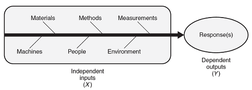
Figure 1: Cause-and-effect diagram depicting inputs (Xs) and outputs (Ys)

Every output/response demonstrates variation. This variation results from variation in the known process variables, variation in the unknown process variables, and/or variation in the measurement of the response variable. This variation is categorized into two categories of special cause variation: unusual responses compared to previous history; and common cause variation, which is variation that has been demonstrated as typical of the process. Common cause variation, also known as the noise of the process, is referred to in experimental design as inherent variation or experimental error.

DOE can help effectively characterize the process (i.e., determine the significant few inputs/settings from among the trivial many inputs/settings). The objectives of a DOE are to learn how to:

• Maximize the output/response
• Minimize the output/response
• Adjust the output/response to a nominal value
• Reduce process variation
• Make the process robust
• Determine which inputs/factors are important to control
• Determine which inputs/factors are not important to control

DOE simultaneously studies several process variables. By combining several variables in one study instead of creating a separate study for each, the amount of testing required is drastically reduced, and greater process understanding will result. This is in direct contrast to the typical one-factor-at-a-time (OFAT) approach, which limits understanding and wastes data. Additionally, OFAT studies cannot be assured of detecting the unique effects of combinations of factors, otherwise known as interactions.

Types of Experiments

There are several types of experiments that can be used to characterize the process by determining the significant few inputs/settings from among the trivial many inputs/settings.

Analysis of Variance (ANOVA) is a basic statistical technique for analyzing experimental data. It subdivides the total variation of a data set into meaningful component parts associated with specific sources of variation, including interactions. In its simplest form, ANOVA provides a statistical test of whether or not the means of three or more groups are equal and therefore generalizes the t-test to more than two groups. ANOVAs are the most useful when comparing three or more means for statistical significance.

Full factorial designs evaluate the combination of all levels of all factors in an experiment. These experiments completely characterize a process. However, full factorial designs can be time consuming and costly due to the number of experimental runs required.

Fractional factorial designs contain a fraction of the number of full factorial runs. The resulting confounding is complete instead of partial. It can be effectively optimized for any number of factors.

One-factor-at-a-time (OFAT) experiments vary each factor individually while holding the levels of other factors constant. For example, an individual tries to fix a problem by making a change, then executing a test. Depending on the findings, something else may need to be tried.

Screening designs provide information primarily on main effects, incurring the risks associated with confounding, in order to determine which of a large number of factors merit further study. As the number of factors increases in a factorial design, the cost and difficulty of control increase even faster due to the acceleration in the number of trials required. Screening designs can be used for as few as four factors or as many as can be practically handled or afforded in an experiment. Their purpose is to identify or screen out those factors that merit further investigation.

Mixture design experiments represent a special type of experiment in which the product is made up of several components or ingredients. This type of experiment is useful in situations involving formulations or mixtures. The output response is related to the proportions of the different components of the formulation or ingredients in the mixture. Mixture experiments depend on the proportions of the formulation or ingredients. The amounts of each component must add up to a total of 1, or 100 percent. Mixture designs are the most useful type of experiment in determining the best composition of a product.

Orthogonal arrays, also known as Taguchi experiments, consist of a set of fractional factorial designs which ignore interaction and concentrate on main effect estimation. These experiments also allow for up to three levels for each factor.

Supporting Statistical Tools And Techniques

There are several basic statistical tools and techniques that are used when performing a DOE. Applying inappropriate methods can invalidate the experiential results.

The Dean and Dixon outlier test is a valid method for detecting outliers when the data is normally distributed. Outlier data points must be evaluated and removed to prevent undue influence on the dependent output(s). If not removed, a factor may be determined to be significant when, in fact, it is not.

Hypotheses testing works with small samples from large populations. Because of the uncertainties of dealing with sample statistics, decision errors are possible. There are two types of errors: type I errors and type II errors. A type I error occurs when the null hypothesis is rejected when it is, in fact, true. In most tests of hypotheses, the risk of committing a type I error (known as the alpha [α] risk) is stated in advance along with the sample size to be used.  A type II error occurs when the null hypothesis is accepted when it is false. If the means of two processes are, in fact, different, and we accept the hypothesis that they are equal, we have committed a type II error. The risk associated with type II errors is referred to as the beta (β) risk. This risk is different for every alternative hypothesis and is usually unknown except for specific values of the alternative hypothesis. Figure 2 is a hypothesis truth table.

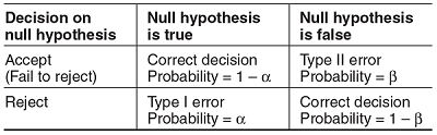
Figure 2: Hypothesis truth table

Normal probability plots can be constructed to look for linearity when using one variable. Normal probability plots provide a visual way to determine if a distribution is approximately normal. If the distribution is close to normal, the plotted points will lie close to a line. Systematic deviations from a line indicate a non-normal distribution:

• Right skew is present if the plotted points appear to bend up and to the left of the normal line; this indicates a long tail to the right
• Left skew is present if the plotted points bend down and to the right of the normal line; this indicates a long tail to the left
• Short tails are present if an S-shaped curve indicates shorter-than-normal tails, that is, less variance than expected

A half-normal probability plot is a graphical tool that uses the ordered absolute estimated effects to help assess which factors are important and which are unimportant. The effects that are not significant will have plotted points that lie close to a line that has its origin at 0,0 and passes through the cumulative percentage point near 50 percent.  Figure 3 is an example half-normal probability plot showing factors A and B are significant.

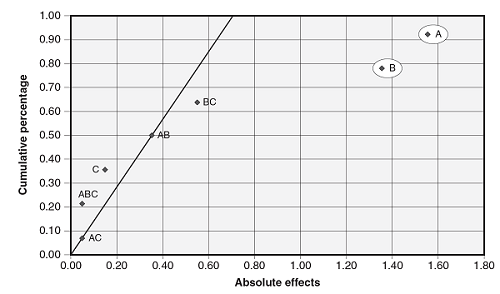
Figure 3: Example half-normal probability plot

Conclusion

DOE is a very powerful tool that can be easily used to characterize a process. DOEs can be performed using a simple inexpensive scientific calculator, spreadsheet, or sophisticated statistical software applications.  There are many resources available online to help learn the fundamentals and application of DOE, many of which are free. Start with simple experiments and, as you gain experience, apply the knowledge gained to more complex problems.

References:

1. Durivage, M.A., Practical Engineering, Process, and Reliability Statistics, ASQ Quality Press, Milwaukee, 2014.
2. Durivage, M.A., Practical Design of Experiments (DOE), ASQ Quality Press, Milwaukee, 2016.
3. Durivage, M.A., “Process Characterization The Foundation For Validation,” Life Science Connect, November 2016.

About The Author:

Mark Allen Durivage has worked as a practitioner, educator, consultant, and author. He is managing principal consultant at Quality Systems Compliance LLC, an ASQ Fellow, and an SRE Fellow. He earned a BAS in computer aided machining from Siena Heights University and an MS in quality management from Eastern Michigan University. He holds several certifications, including CRE, CQE, CQA, CSQP, CSSBB, RAC (Global), and CTBS. He has written several books available through ASQ Quality Press, published articles in Quality Progress, and is a frequent contributor to Life Science Connect. Durivage resides in Lambertville, Michigan. Please feel free to email him at mark.durivage@qscompliance.com or connect with him on LinkedIn.