Calculating The Process Capabilities Of Cleaning Processes: A Primer

By Andrew Walsh, Miquel Romero Obon, and Ovais Mohammad

Part of the Cleaning Validation for the 21st Century series

 

With the publication of the ASTM E3106 Standard¹ in 2017, the pharmaceutical industry began the movement to science-, risk-, and statistics-based approaches to cleaning process development and validation. Due to this movement, process capability has become a critically important measure for demonstrating the acceptable performance of cleaning processes.² Process capability is also vital for measuring the risk associated with these cleaning processes³ and ultimately for determining the level of effort, formality, and documentation necessary for cleaning validation.⁴ Clearly then, an understanding of calculating process capability and how to apply it to cleaning processes is essential to implement the science and risk-based approaches of ASTM E3106. This article will explain what process capability is, the various techniques that can be used for calculating process capability, and how it should be applied to cleaning processes.

Introduction To Process Capability

Process Capability (C_P) is simply the ratio of the spread of the process data (its variability) to the spread of the specifications for that process. Basically, it is a measure of how well the spread of the data can fit within their specification range.  A process is said to be capable when the spread of its data is contained within its specification spread. The smaller the spread of process data is than the specification spread, the more capable a process is. These C_P concepts are illustrated in Figure 1:

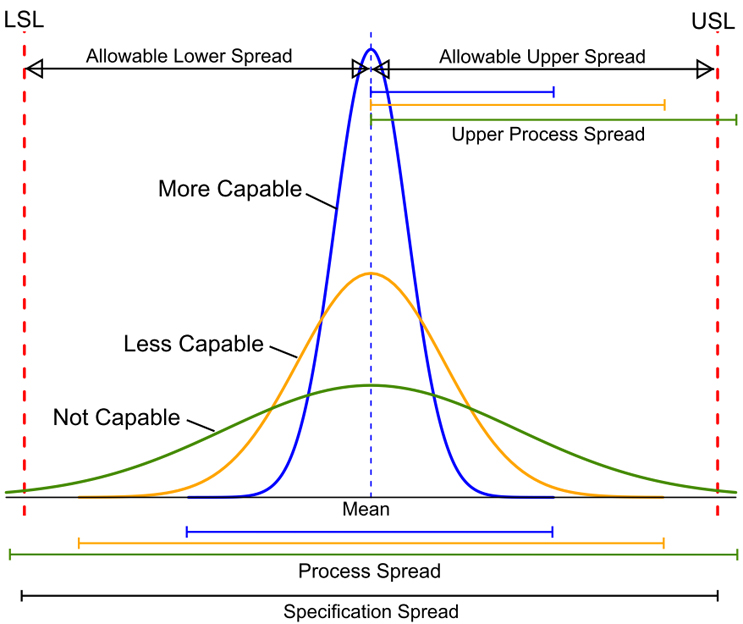
Figure 1: Comparisons of Process Spread to Specification Spread

A number of indices are used as measures of process capability or process potential. Among them are the widely used C_p, C_pk, C_pl, and C_pu. These four standard indices are defined in Table 1 below using the process mean (μ), process standard deviation (σ), lower specification limit (LSL), and upper specification limit (USL):

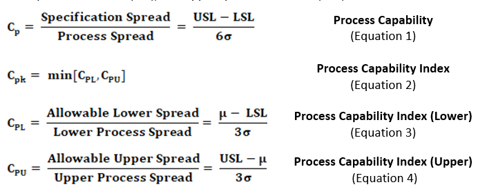
Table 1: Standard Indices of Process Capability

The indices C_p and C_pk are used as capability measures for processes that have both upper and lower specification limits (i.e., the specification limits are two-sided). On the other hand, for processes that only have lower or upper specification limits (i.e., the specification limit is one-sided, such as with cleaning data), C_PL and C_PU are used as measures of their capability and C_p is not. The indices C_PL and C_PU compare the lower and upper spread of the process data to the distance from the data’s center (i.e., mean) to the upper specification limit and to the lower specification limit, respectively. (Note: When working with one-sided specifications, C_pk does not refer to the minimum value of C_PU and C_PL but to whichever the one-sided limit is  upper or lower.)

Figure 2a shows hypothetical data with a mean of 100 and a standard deviation (σ) of 15 analyzed against a specification range of 25 to 175, which results in a C_p of 1.67.  This is a good result. However, data are rarely centered exactly within the specification range and are normally closer to one specification limit than the other. The standard C_p calculation will not reveal this. As an extreme example, Figure 2b shows that 100% of the data can be outside of the specification range and the C_p calculation will be the same. It should be understood that process capability as measured by C_p can only reveal if the process is potentially capable of meeting the specification range — not that it does meet the specification.

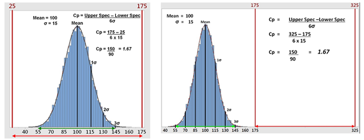
Figure 2a: Example 1 of Process Capability (Cp) - This graph shows hypothetical data with all the data well within the specification range (25 to 175), which yields a C_p of 1.67. Figure 2b: Example 2 of Process Capability (Cp) - This graph shows the hypothetical data but with all the data outside the specification range (175 to 325), which still yields a C_p of 1.67.

An improvement on the C_p calculation that provides better information about the process is the C_pk (process capability index) calculation. The C_pk index has been designed particularly for processes that are not centered within the specification range. This index only looks at the distance of the mean to whichever specification limit is closest to the mean. In these cases, either the C_pu (for upper specification limit (USL)) or C_pl (for lower specification limit (LSL)) is used, and these are simple ratios of the difference of the data’s mean from the upper or lower specification limit to half of the spread of data (its variability).

Figure 3 shows plots and process capability calculations for two hypothetical data sets. The data set on the top has a mean of 100 that is centered between the upper and lower specification limits and a standard deviation of 15. As can be seen, the capability indices C_p and C_pk are the same for these data. Whereas the lower data set in Figure 3 has a mean of 85 that is not centered between the upper and lower specification limits; it has the same standard deviation of 15. In this case, as the mean is shifted toward the lower specification limit, the C_pk value is less than the C_p value. This shift makes the data set look better against its upper specification limit but worse against its lower specification limit.

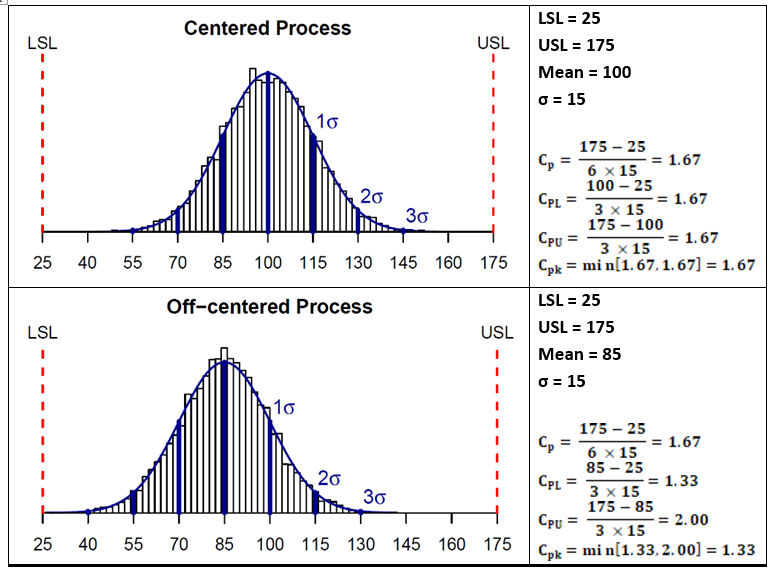
Figure 3: Examples showing calculations of Process Capability indices

Assumptions For Estimating Process Capability

As seen from the formulas above, calculating these process capability indices (PCIs) is simple and straightforward. However, it should be noted that these calculations are based on the assumptions that the process data are normally (or approximately normally) distributed and that the process is stable (the absence of significant trends such as drifts and/or stationarity).

For cases where the process data is not normally distributed or may not be expected to be (e.g., swab results obtained from different locations during a cleaning qualification/verification run where the collection of samples is not done in a particular sequence or order), a different set of indices, known as process performance indices (PPIs), are used for comparing process data to specification limits. These indices, denoted by P_P, P_PK P_PL, and P_PU, are used in place of C_P, C_PK C_PL, and C_PU respectively, to measure compliance to specifications using a detrended estimation of sigma. The formulas for calculating these indices are the same as the ones used for calculating PCIs, the only difference being the type of standard deviation used. In estimating PCIs, group or short-term standard deviation (the one estimated using control charts) is used, whereas overall or long-term standard deviation (i.e., the standard deviation of all the values) is used when estimating PPIs.⁵ Similarly, when the process data are not normally distributed (e.g., microbial data), different formulas that are based on percentiles of the fitted or empirical distribution are used for calculating PCIs or PPIs. These modified indices are interpreted the same way as the standard PCIs discussed earlier. For ease of understanding, only the notations used for standard PCIs will be used in this article.

Requirements For Process Capability

In Six Sigma or Operational Excellence programs, the values generated by these process capability calculations are considered critical in interpreting how acceptable a process is. The guidelines that are widely used for these values are shown in Table 2.

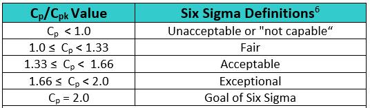
Table 2: Six Sigma Definitions of Process Capability Values

The goal of these so-called "Six Sigma" programs has been to develop or improve manufacturing processes such that they have an additional three standard deviations (sigma) of room on both sides of their process data, which mathematically calculates to a Cp of 2.0. It should be noted that, in practice, many companies have been satisfied just to reach Five Sigma (Cp = 1.66) and feel that striving for Six Sigma (Cp =2.0) is not worth the extra cost and effort. Achieving a process capability of 1.66 is considered very good.

There are other recommended values, depending on the process being measured. For processes with two-sided specifications, Montgomery⁷ recommends minimum values of Cp/Cpk of 1.33 for existing processes, 1.50 for new processes or for existing processes involving a critical attribute/parameter (e.g., safety or strength), and 1.67 for new processes involving a critical attribute/parameter (e.g., safety or strength). For processes with one-sided specifications, he recommends minimum values of Cpu/Cpl as: 1.25 for existing processes, 1.45 for new processes or for existing processes involving a critical attribute/parameter (e.g., safety or strength), and 1.60 for new processes involving a critical attribute/parameter (e.g., safety or strength).

Like other statistical parameters that are estimated from sample data, the calculated process capability values are only estimates of true process capability and, due to sampling error, are subject to uncertainty. Hence, to address these uncertainties, it is prudent to compare lower or upper confidence limits of the estimated process capability indices to the capability requirement when making decisions pertaining to process capability. Almost all statistical software in use today can provide confidence intervals for process capability values. For the two example data sets shown in Figure 3, 95% one-sided lower bounds for C_PU were estimated to be 1.47 (centered process) and 1.75 (non-centered process). Since this value is lower than 2.0, we cannot conclusively infer that the process has met that Six Sigma goal.

Cleaning Process Capability

As we have seen, process capability is an important process performance measure that is relatively simple to calculate, as it only requires the mean and standard deviation of data from the process and the specification limits for that process. So, in the case of a cleaning process, the process capability of the cleaning process can be calculated from the mean and standard deviation of the swab or rinse data from the cleaning process and the Health Based Exposure Limit (HBEL)-based cleaning limits for the swab or rinse data.

To determine process capability (C_pu) of a cleaning process, the terms in this equation can be substituted with the values estimated from cleaning (swab or rinse) data and the HBEL-based cleaning limit as shown in the example in Equation 5.

Statistical software such as Minitab, JMP, "R," and many others are capable of performing process capability analyses and graphing the results, such as the example report in Figure 4.

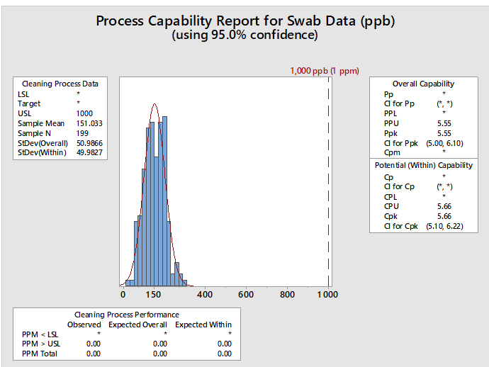
Figure 4: Example of Process Capability Analysis in Minitab for Hypothetical Swab Data - This graph shows the process capability of swab sample data (N=199) with a mean of 151 ppb and a standard deviation of 50 ppb. The hypothetical HBEL-based limit is 1,000 ppb or 1 ppm. The process capability is shown as the process performance upper (PPU) for the overall capability with a value of 5.55 and as process capability upper (CPU) for the potential (within) capability with a value of 5.66. Minitab provides the option of calculating confidence intervals for the process capability values since the mean, standard deviation, and N are all known. This option is especially useful when there is a small number of samples. The confidence intervals for the CPU are 5.10 and 6.22, meaning that based on the number of samples (N), the CPU could be as low as 5.10 or as high as 6.22. The graph also shows the number of observed and expected failures per million (PPM &GT USL) is 0.00.

Also, since process capability values are derived from the mean and standard deviation, upper and lower confidence intervals can be calculated for these process capability indices. In cases where there may be varying or small sample sizes (e.g., where N is typically < 25) it is prudent and recommended to report and use the lower confidence limit of the C_pu from these calculations instead of just the C_pu itself. Almost all statistical software in use today can provide confidence intervals for process capability values. Figure 4 shows an example using Minitab 17. In the textbox on the right, from the output from Minitab reports, the C_pu as 5.66 and additionally reports that the 95% confidence intervals (CI) for the C_pu range from 5.10 to 6.22. (Note: Minitab reports the CI for the C_pk, which is either the C_pu or the C_pl; in this case it is the C_pu.)

Minitab can also report the expected number of failures out of a million based on the process capability analysis. In this example, the lower textbox reports, based on these data, that there are 0.00 possible failures out of 1 million (i.e., exceeding the upper specification limit). This indicates that there is a very low probability of a cleaning failure in this example.

Process Capability Of Non-Normal Data

It is important for the reader to understand that the calculations (in equations 4 and 5) for estimating process capability are based on the assumption that the process data are normally (or approximately normally) distributed. However, not all cleaning data follow a normal distribution. For example, while swab data for total organic carbon analysis are frequently normally distributed, HPLC data are frequently not.  Before performing any statistical analysis of cleaning data, it is important to determine whether the data are normally distributed or not.  If the cleaning data are not normally distributed, the following options can be used in these situations:

1. Transform the data to a Normal distribution. When this strategy is followed, limits should be also transformed accordingly.

• The Box/Cox Transformation (power) raises the data to either the square, the square root, the log, or the inverse.
• The Johnson Transformation selects an optimal transformation function.

2. Identify the data distribution and evaluate the data using a non-normal distribution model.^8,9

• Lognormal, Gamma are some examples

3. Evaluate the data using a non-parametric method.

• Empirical percentile method

When using option 2, it is necessary to identify which of the many non-normal distribution models to use. Minitab has a test (Individual Distribution Identification) that can evaluate data against 12 different and common distributions. Based on these evaluations, the best-fitting distribution model can be selected.  For example, Figure 5 shows a graph generated by Minitab comparing four distributions (normal, lognormal, gamma, and exponential). The data set being analyzed is randomly generated data from a gamma distribution. The interpretation of the graphs is based on a visual examination of how well the data fall along the expected (red) line and whether the P-value of the Goodness of Fit Test for the distribution is greater than 0.05. The red line plots where the data should fall if they follow that particular distribution. If the data do not fall along the red line, then the data are unlikely to be from that distribution. If the data appear to follow the red line, the next criterion to check is the P-value. By convention, the P-value should be greater than 0.05, indicating there is at least a 1:20 chance that the data follow this distribution, and it is considered safe enough to analyze the data using this distribution.

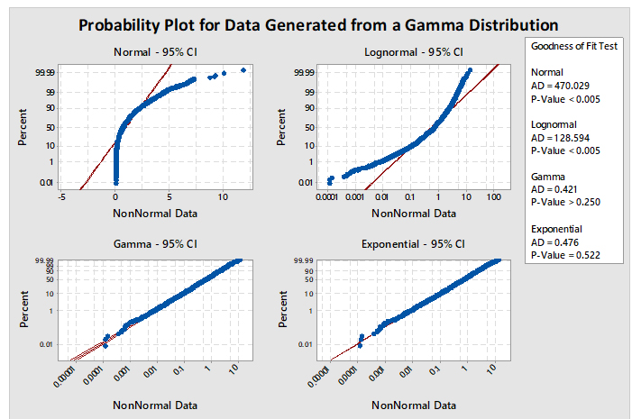
In Figure 5, the plots for the normal and lognormal distributions are clearly off their red lines and also have P-values of <0.005. Consequently, these distributions would be appropriately rejected as good models for analyzing these data. The gamma and exponential plots closely follow their red lines and appear very similar to each other. Examination of their P-values reveals the gamma to be 0.250 and exponential to be 0.522. Both distributions pass the criteria for selection.

But should the exponential distribution be selected since it has the higher P-value even though we know the data came from a gamma distribution? The higher P-value does not indicate that the exponential is the best distribution to select; it only means that the distribution of the data is not significantly different statistically from the exponential distribution and there is just less evidence to reject the exponential distribution as a good fit for the data.  The choice of which distribution to use should be based on where the data were collected from and what type of distribution the data would be expected to follow. It should also be understood that the gamma distribution is actually a "family" of distributions and, depending on its shape and scale parameters, the gamma distribution can closely follow the exponential distribution, which explains the results in Figure 5.

Figure 6 shows process capability analyses of the data from Figure 5 using the gamma distribution (left) and the exponential distribution (right). It is immediately evident that the data are well described by both distributions and the process capability results are basically identical. In this case, and in many other cases, the choice of the distribution model is not critical. In addition, a visual inspection of the data may be helpful when deciding among multiple distributions that statistically fit the data.

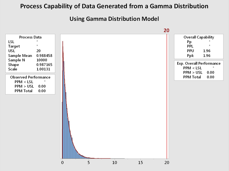
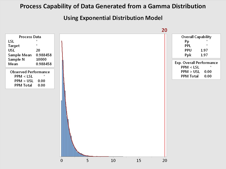
Figure 6: Process Capability Analysis of Data Generated From a Gamma Distribution using Gamma and Exponential Distributions - These graphs show the process capability evaluation of the data set of 10,000 random values generated from a gamma distribution using both gamma and exponential distributions. There is no difference in the analysis of the data. This is due to the data closely fitting both distribution models.

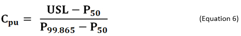
As an alternative to using non-normal distributions, there are different formulas based on percentiles of the fitted/empirical distribution that can be used for calculating process capability. If the distribution of process data is known, or can be assumed, the formula in Equation 6 is used for calculating process capability index Cpu. In the equation, P₅₀ and P_99.865 are the 50^th (median) and 99.865^th percentiles of the specified distribution, respectively.⁶

Similarly, when the underlying distribution of process data is unknown, a non-parametric (distribution-free) variant of Cpu calculated by empirical percentile method proposed by McCormack et al, can be used.⁸ The Cpu calculation using this method is shown in Equation 7. In the equation, P₅₀ and P_99.5 are the 50^th (median) and 99.5^th percentiles of the empirical distribution, respectively.

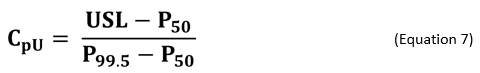
This approach can only be used when sample size is ≥100. A macro for calculating non-parametric capability indices based on McCormack’s approach is available on Minitab’s website.¹⁰

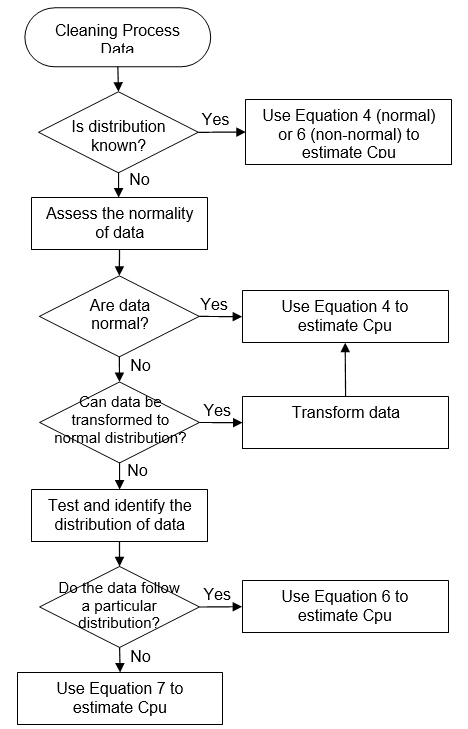
These modified indices are interpreted the same way as the standard Cpu discussed earlier. Examples of decision trees to identify the calculation method for Cpu are given in Appendices I and II.

"All Models Are Wrong, But Some Are Useful"

It may be surprising for some readers to realize, as we saw in Figure 5, that more than one distribution model may be used to analyze data instead of the "correct one." Actually, this is perfectly acceptable as, in truth, there is no "correct one" or "absolutely true" model. The quote starting this section is typically attributed to the statistician George E. P. Box, and this quote is considered famous, primarily among statisticians. 

George E. P. Box expanded on this idea, stating:

"Remember that all models are wrong; the practical question is how wrong do they have to be to not be useful."¹²

Box's comment is most relevant to this article since there are voices in the cleaning validation community claiming that process capability is not appropriate for cleaning or cannot be determined since cleaning data are non-normal or simply that statistics is unnecessary for cleaning. Consequently, there has been hesitancy to adopt these techniques out of fear that the analysis may be calculated incorrectly and serious errors made. However, comparisons of process capabilities calculated using multiple distributions have shown that such errors are minimal if an appropriate selection process has been followed.¹³ Appendices I and II offer two decision trees that can be followed to minimize errors in selecting models.

Conclusion

Many pharmaceutical companies have implemented Six Sigma programs in the past 10 years or more and have come to understand the significance and value of process capability analysis. These companies have also come to understand that process capabilities less than 1.00 are inadequate. They also understand that process capabilities greater than 1.66 are within reach and the benefits of achieving this level of process capability is very much worth the effort. For many cleaning processes it is possible to easily achieve process capabilities of greater than 10! In fact, the suggested values for Six Sigma programs in Table 2 are not appropriate for cleaning processes, as they are easily capable of much higher process capabilities.

The assessment of process capabilities provides important knowledge and understanding about the cleaning process and allows for a quantitative measure of the risk to the patient from carryover of residuals.  Understanding the level of risk that cleaning process capability can provide can also facilitate implementing the second principle of ICH Q9 and justify a "level of effort, formality and documentation commensurate with the level of risk" for the cleaning validation process.⁴ The knowledge and understanding gained from such cleaning process capability estimates can even justify the use of simpler analytical methods such as visual inspection for cleaning verification or validation.^{14, 15}

Peer Review

The authors wish to thank Thomas Altman; Joel Bercu, Ph.D.; James Bergum, Ph.D.; Sarra Boujelben; Alfredo Canhoto, Ph.D.; Gabriela Cruz, Ph.D.; Mallory DeGennaro; Parth Desai; Jayen Diyora; David Dolan, Ph.D., DABT, Kenneth Farrugia; Andreas Flueckiger, M.D.; Christophe Gamblin; Ioanna-Maria Gerostathes; Ioana Gheorghiev, M.D.; Jessica Graham, Ph.D.; Laurence O'Leary; Prakash Patel; Kailash Rathi; Stephen Spiegelberg, Ph.D.; and Basundhara Sthapit, Ph.D.; for reviewing this article and for providing insightful comments and helpful suggestions.

References

1. American Society for Testing and Materials (ASTM) E3106-18, "Standard Guide for Science-Based and Risk-Based Cleaning Process Development and Validation," www.astm.org.
2. Walsh, Andrew, Ester Lovsin Barle, David G. Dolan, Andreas Flueckiger, Igor Gorsky, Robert Kowal, Mohammad Ovais, Osamu Shirokizawa, and Kelly Waldron, "A Process Capability-Derived Scale For Assessing Product Cross-Contamination Risk In Shared Facilities," Pharmaceutical Online August 2017
3. Walsh, Andrew, Thomas Altmann, Alfredo Canhoto, Ester Lovsin Barle, David G. Dolan, Andreas Flueckiger, Igor Gorsky, Jessica Graham, Ph.D., Robert Kowal, Mariann Neverovitch, Mohammad Ovais, Osamu Shirokizawa and Kelly Waldron, "Measuring Risk in Cleaning: Cleaning FMEA and the Cleaning Risk Dashboard," Pharmaceutical Online April 2018
4. Walsh, Andrew, Thomas Altmann, Ralph Basile, Joel Bercu, Ph.D., Alfredo Canhoto, Ph.D., David G. Dolan Ph.D., Pernille Damkjaer, Andreas Flueckiger, M.D., Igor Gorsky, Jessica Graham, Ph.D., Ester Lovsin Barle, Ph.D., Ovais Mohammad, Mariann Neverovitch, Siegfried Schmitt, Ph.D. and Osamu Shirokizawa, "The Shirokizawa Matrix: Determining the Level of Effort, Formality and Documentation in Cleaning Validation," Pharmaceutical Online December 2019
5. ASTM E2281-15(2020), Standard Practice for Process Capability and Performance Measurement, ASTM International, West Conshohocken, PA, 2020, www.astm.org
6. T. Pyzdek, “The Six Sigma Handbook,” 2003, McGraw Hill
7. Montgomery, D. C., “Introduction to Statistical Quality Control,” 7th Edition (2012), John Wiley & Sons, Inc.
8. ISO/TR 22514-4 (2007) “Statistical methods in process management – Capability and performance - Part 4: Process capability estimates and performance measures”.
9. D. W. McCormack, Jr., Ian R. Harris, Arnon M. Hurwitz & Patrick D. Spagon (2000) “Capability Indices for Non-Normal Data”, Quality Engineering, 12:4, 489-495, DOI: 10.1080/08982110008962614
10. Cathy Akritas, Macro: ECAPA.MAC, Non-parametric capability analysis, available at https://support.minitab.com/en-us/minitab/18/macro-library/macro-files/quality-control-and-doe-macros/non-parametric-capability-analysis/ (as of 09/09/2021)
11. Chang, P.L. and Lu, K.H. (1994) PCI Calculations for Any Shape of Distribution with Percentile. Quality World, Technical Section, 20, 110-114.
12. Box, George E.P. and Norman R. Draper "Empirical Model-Building and Response Surfaces," ‎Wiley; 1st edition (January 1, 1987)
13. Walsh, Andrew, "Cleaning Validation - Science, Risk and Statistics-based Approaches," 1st Edition (2021) ISBN: 978-0-578-89661-8
14. Desai, P., and Walsh, A., “Validation of Visual Inspection as an Analytical Method for Cleaning Validation,” Pharmaceutical Online, August 2017.
15. Andrew Walsh, Ralph Basile, Ovais Mohammad, Stéphane Cousin, Mariann Neverovitch, and Osamu Shirokizawa, "Introduction To ASTM E3263-20: Standard Practice For Qualification Of Visual Inspection Of Pharmaceutical Manufacturing Equipment And Medical Devices For Residues," Pharmaceutical Online January 2021

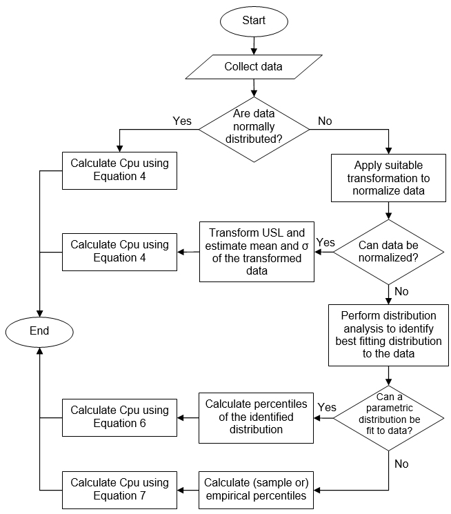
Appendix I

Decision Tree to Identify the Calculation Method for Cpu (Example 1)

Appendix II

Decision Tree to Identify the Calculation Method for Cpu (Example 2)