Calculating Process Capability Of Cleaning Processes: Analysis Of Total Organic Carbon (TOC) Data

Part of the Cleaning Validation for the 21st Century series

Our previous article provided background on the concept of process capability and how it could be used to measure the risk associated with cleaning processes.¹  This article will examine a data set of actual total organic carbon (TOC) swab data collected during cleaning validation for a pharmaceutical manufacturing facility and will show how much cleaning process knowledge and cleaning process understanding can be easily obtained through some simple statistical evaluations of such data.

This analysis will also reveal how the adoption of cleaning process capability as a measure of cleaning risk will not allow for the "relaxation of cleaning efforts," which has been a concern of regulators with the implementation of the health-based exposure limit (HBEL) after the EMA abandoned the historical non-health-based approaches (i.e., 0.001 lowest therapeutic dose and 10 ppm).

Background On The TOC Data Set

The TOC data set used in this analysis was collected from filling equipment for semi-solid pharmaceutical products. TOC is potentially the ideal analytical method for evaluating the cleanliness of equipment surfaces as it will detect almost any possible source of organic carbon present on the equipment. Since the vast majority of pharmaceutical substances/products (active pharmaceutical ingredients, excipients, etc.) contain significant amounts of organic carbon, TOC can be used to detect all these compounds in one analysis. TOC can also detect residues of any cleaning agents containing organic carbon. The sensitivity of some TOC instruments is in the very low parts per billion (ppb or μg/mL) range, so there is always a possibility of detecting low organic carbon signals in cleaning samples even after scrupulous cleaning. This also makes TOC data potentially amenable to statistical analysis, including process capability analysis and statistical process control.

These TOC data were collected from four filling lines, and there was one cleaning SOP (manual cleaning) used for all the filling equipment in this study. This data set consisted of 155 swab samples taken from multiple sites on this filling equipment after cleaning, ranging from nine to 13 samples per cleaning run. Figure 1 shows an example diagram of one filling line with a typical sampling scheme.

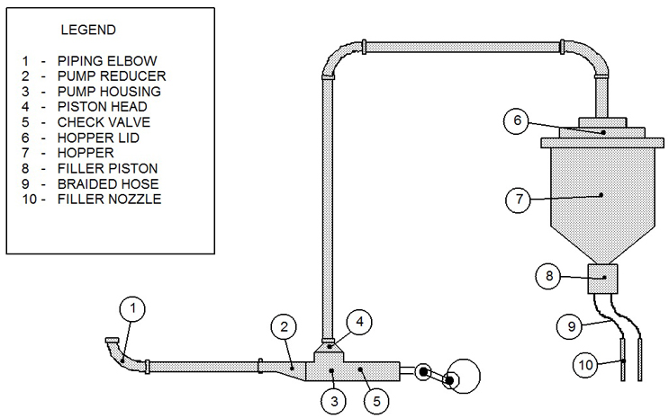
Fig. 1 - Example Diagram of Sample Sites for a Filling Line

The intent was to use these data to determine the process capability of the cleaning process and then set a statistical process control (SPC) limit for TOC swab results. Initially, these data were given to a company statistician for analysis. Figure 2 shows an empirical probability density plot that was created by the statistician. The bulk of the data appeared to be normally distributed with a small tail of data to the right. However, the statistician reported back that these data were not normally distributed. The statistician suggested that an upper control limit (UCL) of 900 ppb could be set based on the 95th percentile of the data.

Fig. 2 - Empirical Probability Density Plot of TOC Swab Data - Data is in parts per billion (ppb).

Consequently, it was decided to set the UCL at 1,000 ppb, or 1 ppm. A limit of 1 ppm was deemed appropriate based on the fact that all of the data were in the ppb range, with few, if any, data ever in the ppm range. Additionally, the experience of collecting TOC data had made 1 ppm a "psychological threshold" between typical and suspect data. And, finally, 1 ppm was easy to remember as well as being statistically justifiable.

That was the extent of the statistical analysis of these data at the time. However, the advent of Six Sigma and Process Excellence programs has brought statistical knowledge and understanding to pharmaceutical manufacturing, along with access to powerful statistical software such as Minitab JMP and the R programming language. The tools and techniques of these programs greatly simplify the sophisticated analysis of data sets like these, as we will see below.

Using Six Sigma Approaches To Evaluate The TOC Data

In the Measure phase of the Six Sigma DMAIC process, the first step is a "first pass analysis," where an initial look is taken of the collected data to see what they can tell you about your process. Such a first pass analysis should always be a graphical one, as this can quickly reveal important information about your data. In Six Sigma programs, it is recommended that you "slice and dice" the data until these analyses reveal something to you. In our first pass, a simple histogram, a box plot, and a probability plot were created.

Figure 3 shows a histogram of the TOC data set (with a corresponding box plot above it) that was generated using the R programming language. A visual examination of the histogram reveals that the majority of the data may be normally distributed in a narrow range around 150 ppb, along with a number of outlier data points. In the box plot, the mean (solid blue vertical line) and the median (dotted blue vertical line) indicate that these data are skewed somewhat to the right (the mean is greater than the median) and identifies the suspected outliers in the histogram as actual outliers (circles). At the time of these studies, these outliers were considered to be "hot spots" where the cleaning had not been as effective as for the majority of the sample locations.

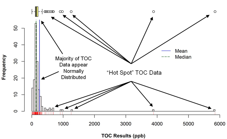
Fig. 3 - Histogram (with Marginal Box Plot) of TOC Data with "Hot Spots"

Figure 4 shows a normal probability plot of these TOC data for a normal distribution, which reveals that these TOC data are not normally distributed. This probability plot compares the percentile ranks of the TOC data against the percentile ranks of the normal distribution. The TOC data points should visually fall along the red line.²

The Anderson-Darling test was chosen to evaluate the data for the normal distribution analysis, as it is known to be more effective in detecting departures in the tails of a distribution. The resulting P-value for the Anderson-Darling test was <0.005, so one would reject the null hypothesis that these data were normally distributed.

Fig. 4 - Probability Plot of TOC Data with "Hot Spots"

It may well be expected that TOC data should be normally distributed as they are the sums of multiple independent random variables (residue variability, sampling variability, dilution variability, analytical variability, etc.), which, according to the Central Limit Theorem, will tend toward normal distributions.³ While the majority of these TOC data appeared to be normally distributed in the probability density plot in Figure 2, the probability plot in Figure 4 clearly indicates that they are not, both visually and using a formal statistical test for normality. This departure from normality is, in all likelihood, due to the presence of these "hot spots" or outlier data points. This is our first indication that these data are not exhibiting random variability ("common cause") and that there is/are some "special cause(s)."

Although none of these data points actually failed the cleaning validation acceptance criteria used at that time, these "hot spots" were very noticeable and were considered substantially different from the other data collected. In fact, during the course of these studies, it became an expectation that all TOC data should be in the range of 100 to 250 ppb (within the normal-looking data seen in Figure 3) and any data above 1 ppm were not expected and, if seen, were immediately suspicious.

These TOC data, including the "hot spots"/outliers, were analyzed for their process capability using an upper specification limit of 1,000 ppb (1 ppm). The 1 ppm limit was chosen for this analysis for demonstration purposes because it had been previously suggested as an upper control limit. The graphical output of Minitab is shown in Figure 5.

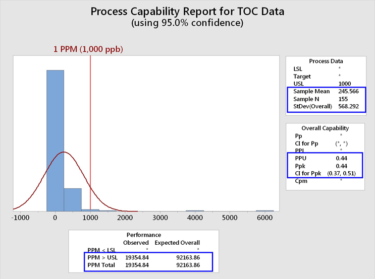
Fig. 5 - Process Capability Analysis of TOC Data Set with "Hot Spots" - The Minitab report lists the PPU (process performance upper) rather than the Cpu (process capability upper). Note that a confidence interval (CI) for the process capability can also be calculated. At the 95% confidence level, the lower bound (LB) is 0.38. It should be considered a good cleaning validation practice to report the LCI as this represents the worst possible case based on the sample size.

(Note: The shape of the histogram appears to indicate non-normal data.)

(Note: CPU is based on the subgroup standard deviation and PPU is based on the overall standard deviation.)

This analysis shows that the mean of these data was 245 ppb, with a standard deviation of 568 ppb. It should be immediately noticed that the standard deviation is more than twice the value of the mean, which corresponds to a relative standard deviation (%RSD) of 232%! The values of the mean and especially the standard deviation have been significantly affected by these "hot spot"/outlier data, resulting in an upward shift in the value for the mean and a severely magnified value for the standard deviation. As the mean and standard deviation are used in the process capability calculation, the process capability has been significantly affected as well.

We can see that the process performance capability (Ppk/PPU) is less than 1 (0.44). As the number of samples (N) is also available, depending on the expectation set for process capability, a lower one-sided confidence bound can also be calculated for this process capability index. In this case we see a LB of 0.38. A value of 1 is considered inadequate in Six Sigma programs and requires remediation. The process capability value must be at least 1.33 to be considered acceptable. This process capability value of 0.44 also resulted in an expected cleaning performance of 92,164 failures per million samples, or over 9 percent of the time, which is clearly unacceptable.

As noted above, this data set would not be considered normally distributed, mostly due to these outlier values. It is generally not considered legitimate to perform statistical analyses that assume a normal distribution on non-normal data. There are several options that can be used in these situations:^4,5

1. Transform the data to a normal distribution. (Note: When this strategy is followed, any limits for the data should also be transformed.)

• The Box-Cox transformation raises the data to either the square, the square root, the log, or the inverse.
• The Johnson transformation selects an optimal transformation function.

2. Identify the data distribution and evaluate the data using a non-normal distribution model., e.g., lognormal, gamma distributions.
3. Evaluate the data using a non-parametric method., e.g., empirical percentile method.

We will examine all three options.

Data Transformation

Both Box-Cox and Johnson transformations were used to transform the TOC data to normality. Figures 6a and 6b show the TOC data after Box-Cox and Johnson transformations, respectively.

Fig. 6a and 6b - Process Capability Analysis of TOC Data Set with "Hot Spots" after (a) Box-Cox Transformation and (b) Johnson Transformation  

* USL was transformed along with the data

For the Box-Cox transformation, the equation X(λ) = (X^λ – 1)/ λ was used for transforming the data and the upper specification limit (USL) of 1,000 ppb using the lambda (λ) value of 0.1. The process capabaility has improved (0.74), as well as the lower bound (0.65), but both are still well below the capability requirement of 1.33. This process capability value of 0.74 also indicates an expected cleaning performance of 13,570 failures per million samples, or over 1 percent of the time, which is still unacceptable.

For the Johnson transformation, the optimal equation in the title of the graph (Figure 6b) was used to transform each data point as well as the USL that was used (1,000 ppb) and this resulted in data that had the best fit for a normal distribution. The process capability is 0.67, with a lower bound of 0.59, but both are still well below the value of 1.33. This process capability value of 0.67 indicates an expected cleaning performance of 22,011 failures per million samples, or over 2 percent of the time, which is still unacceptable.

Non-Normal Distribution

To identify a best-fitting distribution for the TOC data, the Individual Distribution Identification feature of Minitab was used. Based on the goodness of fit (GOF) test results, none of the parametric distributions fit the data well. The GOF results are shown in Table 1. As seen in the table, the P-value of 0.265 (&GT0.05) suggests that the Johnson transformed data fit the normal distribution well.

Table 1: Goodness of Fit Test Results for Distribution Identification

AD = Anderson-Darling, LRT P = Likelihood-Ratio Test (low LRT P values indicate that the fit is improved by the addition of a second or third parameter to the model)

For comparison purposes, the process capability was evaluated assuming lognormal and gamma distributions for the data.

Figure 7 shows the TOC data evaluated using a lognormal distribution.

Fig. 7 - Process Capability of TOC Data Set with "Hot Spots" Lognormal Distribution - a lognormal distribution is a probability distribution of variables whose logarithms follow a normal distribution. Many data follow a lognormal distribution.

The process capability using the lognormal (0.68) is almost identical to the value obtained by the Johnson transformation (0.67) and is also well below the value of 1.33. This process capability value of 0.68 also indicates an expected cleaning performance of 19,355 failures per million samples, or almost 2 percent of the time, which again is unacceptable.

Figure 8 shows the TOC data evaluated using a gamma distribution.

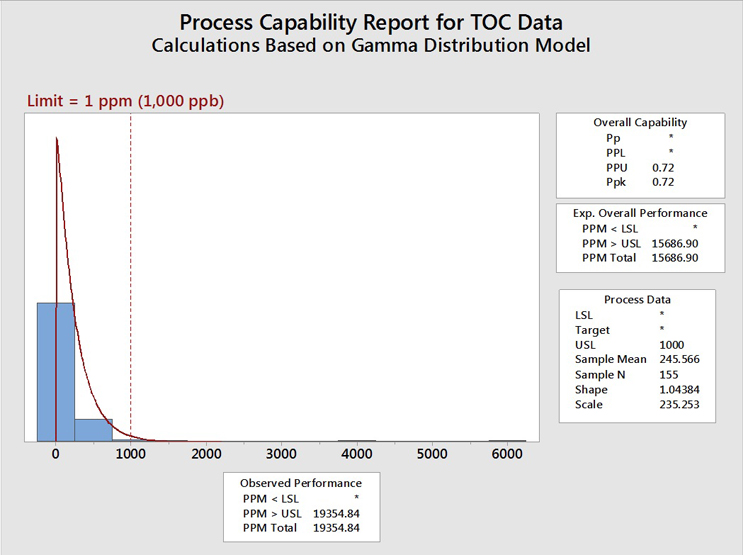
Fig. 8 - Process Capability of TOC Data Set with "Hot Spots" using the Gamma Distribution - Gamma distributions are a family of right-skewed, continuous probability distributions (exponential, Erlang, and chi-squared distributions) and are useful in situations where something has a natural minimum of 0, or a lower boundary, such as is often found with cleaning analytical data.

The process capability assuming a gamma distribution (0.72) is somewhat better (higher) than the values obtained assuming the Johnson transformation (0.67) or the lognormal distribution (0.68) but is still well below the value of 1.33. This process capability value of 0.72 also resulted in an expected cleaning performance of 19,355 failures (same as the lognormal) per million samples, or almost 2 percent of the time, which, again, is still unacceptable.

Non-Parametric Method

For the process capability using a non-parametric approach (empirical percentile method), the data were imported into Excel and the calculations performed as shown in Table 2. This approach yielded a process capability of only 0.21, which is the worst of the four approaches.

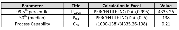
Table 2 - Process Capability by the Empirical Percentile Method using Excel

Table 3 summarizes the process capabilities of each of these approaches and the P-values calculated for the GOF for the distributions.

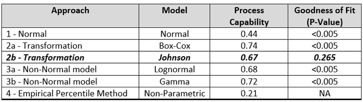
Table 3- Process Capability Values and Goodness of Fit P-Values for Different Approaches

Interestingly, there is very little difference in the process capabilities calculated using the Johnson transformation and either of the non-normal distributions. However, only the Johnson transformation had an acceptable P-value (0.265), indicating the transformed data fit the normal distribution well, so this analysis would typically be the one chosen.

Evaluation Of TOC Data Using The Process Capability Scale

A scale from 1 to 10 for potential use in cleaning FMEAs has been developed that derives scores on a scale directly from the cleaning process capability (C_pu).⁶ This calculation is performed by simply taking the reciprocal of the C_pu and multiplying by 10 (Figure 9).

Fig. 9 - Process Capability Scores for TOC Data Set with "Hot Spots”

Process Capability Score  =  1/C_pu x 10

In the development of this process capability scale, the midpoint was set to a score of 5. This score corresponds to a process capability of 2, which is equivalent to "Six Sigma" in Operational Excellence programs. Scores greater than 5 on this scale are considered increasingly poorer than Six Sigma and scores lower than 5 are considered increasingly better than Six Sigma.

The results of the process capability analysis for the TOC data above were analyzed and resulted in scores ranging from 13.9 to 22.7, all of which are extremely poor and off the top of the scale. The score for the empirical percentile method (48.7) was too far off the chart to plot. Such results indicate, regardless of the data distribution model used, that cleaning improvements are absolutely necessary.

Evaluation Of TOC Data Using The Shirokizawa Matrix

An additional approach has also been developed using the toxicity scale⁷ and the process capability scale⁶ for determining the level of effort, formality, and documentation (as suggested in the 2021 draft ICH Q9 (R1)) necessary for cleaning validation based on the level of risk. The toxicity scale and the process capability scale have been combined into a matrix called the Shirokizawa Matrix.⁸ The toxicity score of a product and the process capability score for its cleaning process can be plotted on this matrix. Eight groupings have been created in the matrix that suggest a level of effort, formality, and documentation necessary for cleaning validation based on the location of the plotted point (Figure 10).

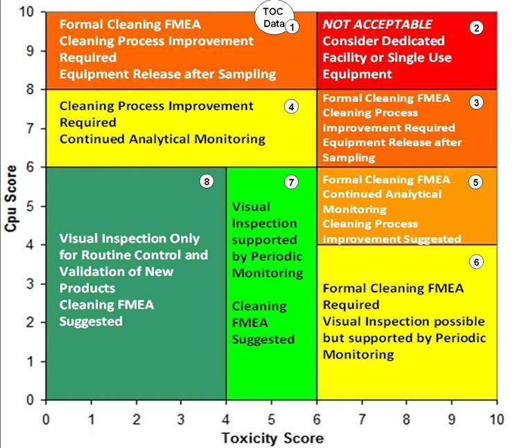
Fig. 10 - Shirokizawa Matrix for TOC Data Set with Hot Spots. Note: The location of the circle labeled "TOC Data" is deceptive as this point is actually far off the process capability scale and the data cannot be plotted on this matrix.

As seen in Figure 10, the process capability score for the TOC data puts it at (actually, off) the top of the scale and corresponds to Group 1 or Group 2 of the Shirokizawa Matrix. Toxicity scores of &GT6 up to 10 (Group 2) would require dedicated facilities or equipment and toxicity scores of <6 down to 1 (Group 1) would require extensive cleaning validation efforts. Neither of these are desirable options, especially considering these were topical formulations of low-hazard compounds. In such situations, cleaning process improvements are clearly necessary. The ASTM E3106 Standard discusses risk reduction activities, including cleaning process development, and these activities should be undertaken in situations such as this.

Importance of Cleaning Process Improvement

We will now examine why cleaning process improvements are not only required of companies in situations like this but should be highly desirable for all companies to perform.  What if cleaning process improvements had been performed on the cleaning process and these "hot spots" no longer occurred?

To explore this question, these "hot spot" data (all data above 400 ppb) were reviewed to determine where and when they occurred and if there were any relationships that could help guide the improvement with the cleaning process. These "hot spots" are shown in Table 4.

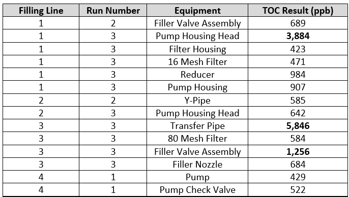
Table 4 - TOC "Hot Spots" - The table shows what filling line the "hot spots" occurred on, what run they occurred on, what equipment they occurred on, and the TOC result for that sample.

There were 14 "hot spot" data points that occurred during a total of 13 qualification runs that were performed for this cleaning process. These "hot spots" occurred on all four filling lines, across the three or four qualification runs for each line, and on 12 different pieces of equipment. Of the 14 "hot spots," 12 were on different pieces of equipment and only two locations had repeated high results (pump housing head and the filler valve assembly). The pump housing head was considered an "easy to clean" piece of equipment and the filler valve assembly was considered a "hard to clean" piece of equipment. It was observed during these qualification studies that these "hot spots" were not specifically associated with hard to clean pieces of equipment and could occur anywhere, including on surfaces that were considered easy to clean.

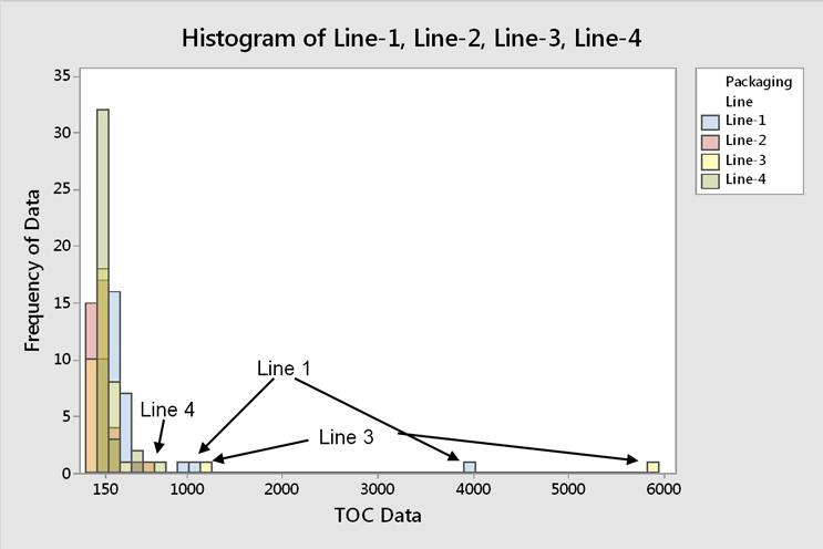
Fig. 11 - Histogram of TOC Data for all Four Filling Lines -"Hot spot" data occur across all four filling lines, while the majority of TOC data are around 150 ppb.

The "hot spot" data were found to occur across all filling lines (Figure 11). It was also observed that pieces of equipment that would typically be considered hard to clean tended to have the lowest results. This may indicate that the operators focused more attention on the hard to clean pieces of equipment, giving less attention to the "easy to clean" pieces of equipment, which resulted in these "hot spots" occurring sporadically. These "hot spots" were also not associated with any particular piece of equipment, so this was not a specific equipment design issue (Figure 12).

Fig. 12 - Histogram of TOC Data for Filling Equipment - "Hot spot" data occur across all pieces of equipment, while the majority of TOC data are around 150 ppb.

These "hot spots" were also not associated with any particular product, as different products were used in the qualification runs on the different lines. The results for the other equipment and for the other runs were very low.

One particular run on Line 1 had five "hot spots." This leads to the conclusion that while the cleaning process was quite capable of cleaning this equipment acceptably, the cleaning performance was variable from run to run. So, in these cleaning studies, operator variability seemed to possibly present an issue and proper training could resolve this. In other words, this poor process capability appears to be something that could be improved.

To observe what effect cleaning improvements would have on the process capability, these 14 "hot spot" data points were removed from the data set and the process capability analyses were performed again. Also of interest is where in the Shirokizawa Matrix such improvements would locate the improved cleaning process and what effect this would have on the level of qualification efforts necessary. Figure 13 is a histogram of the data set with the 14 "hot spots" removed.

Fig. 13 - Histogram of TOC Data "Cleaned" of "Hot Spots"

The mean of these data was reduced to 143 ppb, with a standard deviation of only 70 ppb now. The standard deviation is now half the value of the mean, which corresponds to a relative standard deviation (RSD) of 49%. Clearly, the data appear much more normally distributed without these data.

Figure 14 shows a process capability analysis of these TOC data cleaned of the "hot spots."

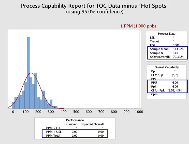
Fig. 14 - Process Capability Analysis of TOC Data Set "Cleaned" of "Hot Spots"

While the RSD is still large, the mean and standard deviation have been positively affected by the removal of these "hot spots." The process capability (Ppk/PPU) is now 4.06 with an LCI of 3.58. This process capability resulted in an expected cleaning performance of 0.00 failures per million samples, or less than 1 in 100 million samples.

Fig. 15 - Normality Test of TOC Data "Cleaned" of "Hot Spots"

Although the data visually appear normal, with the data falling much better along the probability plot, the P-value for the Anderson-Darling test (Figure 15) still indicates a low probability of normality (<0.005 instead of &GT0.05).

It is well known that the normality test is very sensitive to outliers, or any abnormalities in the data set, which can result in low P-values, and false rejection of the null hypothesis, in these cases.  A visual examination of the histogram (Figure 13) and the probability plot (Figure 15) reveals what appears to be possible curvature in several places, so it was suspected that the data set may actually consist of bimodal, or even multi-modal, data. JMP software was used to perform both Normal 2 Mixture Distribution and Normal 3 Mixture Distribution analyses on the data set (Figure 16).

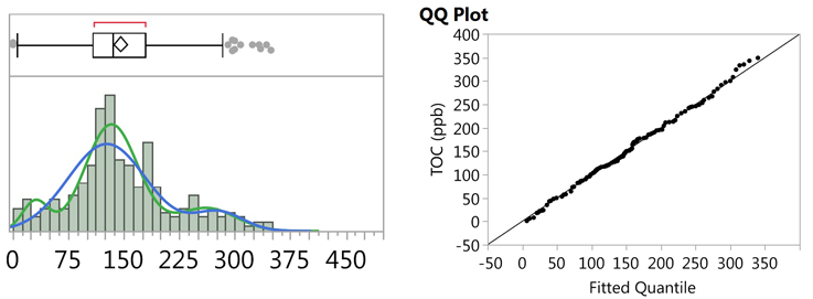
Fig. 16 - Fitted Normal 2 and 3 Mixture Plots and QQ Plot for "Cleaned" TOC Data

Figure 16 shows the fitted plot, which shows the possible presence of three normal distributions within the data set. The quantile-quantile (QQ) plot shows strong normality for these three distributions. JMP also estimates a separate mean and standard deviation and a proportion of the whole for each distribution (Table 5).

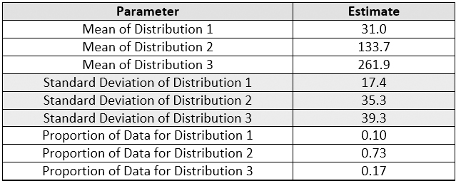
Table 5 - Parameters and Estimates of the Normal 3 Mixture Distributions

Since this analysis provides the parameters for each distribution, these can be used to identify the individual results belonging to these possible distributions and allow an exploration of these data that could potentially identify the source of these distributions.

The means ± 3 standard deviations for Distribution 1 (low data) and Distribution 3 (high data) were calculated, and those parts whose TOC data were found between these means ± 3 standard deviations were tabulated, along with the line and run number they were from (Table 6). This analysis could reveal which pieces of equipment, what lines, or which runs resulted in the low data for Distribution 1 or the high data for Distribution 3.

Table 6 - Parts, Lines, and Runs Associated with Distribution 1 and Distribution 3

A review of the data in Table 6 did not identify any particular parts associated with Distribution 1 (low TOC) or Distribution 3 (high TOC). The same parts showed up in both distributions fairly equally.

Comparison of the lines revealed that Distribution 1 (low TOC) was associated with line 1 and line 4 at 38% and 46% of the time, respectively. Distribution 3 (high TOC) was associated with line 2 and line 3 at 38% and 29% of the time, respectively. If there was an equal probability, then each line would be expected to be 25%. The same "hardest-to-clean" product was used for the qualification runs for line 1 and line 4, which may explain why their results were similar. Different products were used for lines 2 and 3.

Comparison of the runs revealed that Distribution 1 (low TOC) was strongly associated (75%) with run 1 for all lines. Distribution 3 (high TOC) was associated with runs 2 and 3 at 48% and 43% of the time, respectively, for a total of 91%. These results could indicate a higher sense of importance by the operator and more careful cleaning during the first qualification runs resulting in the lower TOC data for these runs. This may have been an example of the so-called "Hawthorne Effect," in which workers are more productive when they know they are being observed.⁹ While there has been some doubt cast on this phenomenon in recent times,¹⁰ this might provide some explanation for the discrepancy between the results for the first runs and subsequent runs. While there were no metadata (e.g., shift, operator, analyst, etc.) collected during these studies that could demonstrate that this phenomenon had occurred, this phenomenon should be considered when designing monitoring or verification programs for cleaning processes.

Taking the process capability results for the data "cleaned" of the 14 "hot spot" data points and plotting it on the Cpu-based process capability scale, we can see that the score is now 2.5 on the scale (Figure 17). This is well beyond a Six Sigma process and can be considered excellent cleaning and a low risk to patient safety.

The process capability score for the TOC data "cleaned" of "hot spots" locates it toward the bottom of the scale now (Cpu Score = 2.5), and this result was plotted on the Shirokizawa Matrix (Figure 18) to determine what the suggested level of effort, formality, and documentation should be at this level of process capability.

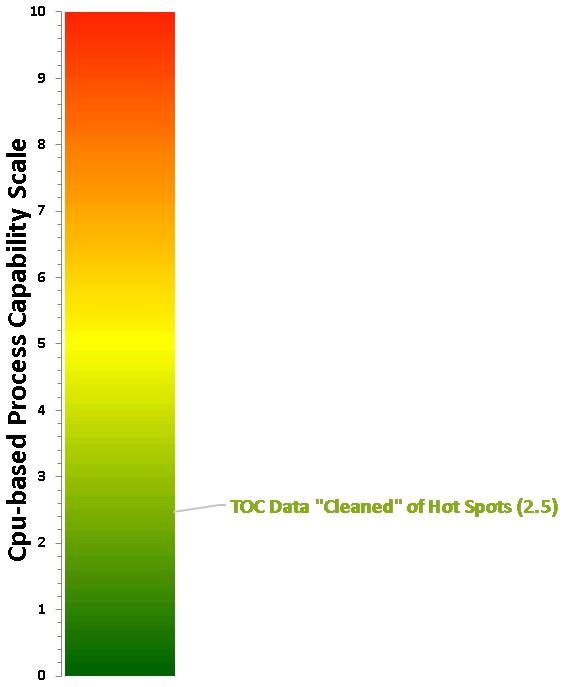
Fig. 17 - Process Capability Score for TOC Data Set with "Hot Spots" Removed

Plotting this process capability score on the Shirokizawa Matrix (Figure 18), we find that the TOC data now falls into Group 6 for toxicity scores of &GT6 up to 10, which would require visual inspection supported by periodic monitoring, and into Groups 7 and 8 for toxicity scores of <6 down to 1, which would also require only visual inspection supported by periodic monitoring. These are highly desirable options, again considering these were topical formulations of low-hazard compounds.

Fig. 18 - Shirokizawa Matrix for TOC Data Set "Cleaned" of Hot Spots

The options in the Shirokizawa analysis in Figure 18 for the "cleaned" TOC data are clearly very desirable. But these options can only be justified through excellent process capability results, which requires excellent cleaning processes, which in turn requires excellent cleaning process development.  Cleaning process development studies as required in the ASTM E3106 Standard, in combination with risk reduction activities, can help companies achieve such results and justify these simpler control strategies.

Clearly, any cleaning process improvement work that can eliminate variability, or "hot spots" such as were found in these data, reduces the risk of cross contamination that could potentially impact patient safety. And any such results as were found in Figure 10 indicate that cleaning process improvements absolutely must be undertaken.

Summary

The TOC data set examined in this article is clearly much more complex than a cursory examination of a simple probability distribution graph, such as in Figure 2, can reveal. If the statistical tools used in this analysis were available at the time that these data were generated, a deeper investigation of the causes for the outliers and the multi-modal nature of the data could have been revealed. And if additional metadata had been collected along with the swab samples, an even deeper analysis would have been possible.

One of the goals of the ASTM E3106 Standard Guide was to provide a framework for implementing the ICH Q9 Quality Risk Management and FDA's Process Validation approaches for cleaning processes. The calculation of process capability is an important part of the risk assessment of cleaning processes and is consistent with ICH Q9 and FDA's 2011 guidance. As stated above, ASTM E3106 Standard provides guidance on performing cleaning process development studies, and excellent process capabilities are easily within the grasp of any company willing to make the effort. If industry and regulators adopt the Shirokizawa Matrix and its control strategy concepts, then companies unwilling to make the effort to improve their cleaning will be required to expend considerable effort on continuing cleaning qualification/verification activities. Therefore any "relaxation of cleaning efforts," as some regulators have feared, should come with significant operational costs to those companies.

Peer Review

The authors wish to thank James Bergum, Ph.D, Joel Bercu, Ph.D., Sarra Boujelben, Gabriela Cruz, Ph.D., David Dolan, Ph.D., Mallory DeGennaro, Parth Desai, Jayen Diyora, Kenneth Farrugia, Andreas Flueckiger, M.D., Christophe Gamblin, Ioanna-Maria Gerostathes, Ioana Gheorghiev, M.D., Igor Gorsky, Jessica Graham, Ph.D., Laurence O'Leary, Ajay Kumar Raghuwanshi, Kailash Rathi, Siegfried Schmitt, Ph.D., and Basundhara Sthapit, Ph.D., for reviewing this article and for providing insightful comments and helpful suggestions.

References

1. Walsh, Andrew, Miquel Romero Obon and Ovais Mohammad "Calculating The Process Capabilities Of Cleaning Processes: A Primer" Outsourced Pharma, November 1, 2021.
2. Ghasemi, A., & Zahediasl, S. "Normality tests for statistical analysis: a guide for non-statisticians". Int J Endocrinol Metab, 10(2) 2012
3. Lyon, Aidan, "Why are Normal Distributions Normal?" Brit. J. Phil. Sci. 65 (2014), 621–649
4. Pyzdek, Thomas “The Six Sigma Handbook” 2nd Edition 2003 McGraw Hill
5. Johnson, Lou ”Modeling Non-Normal Data Using Statistical Software” R&D Magazine August 2007
6. Walsh, Andrew, Ester Lovsin Barle, David G. Dolan, Andreas Flueckiger, Igor Gorsky, Robert Kowal, Mohammad Ovais, Osamu Shirokizawa, and Kelly Waldron. "A Process Capability-Derived Scale For Assessing Product Cross-Contamination Risk In Shared Facilities" Pharmaceutical Online August 2017
7. Walsh, Andrew, Ester Lovsin Barle, Michel Crevoisier, David G. Dolan, Andreas Flueckiger, Mohammad Ovais, Osamu Shirokizawa, and Kelly Waldron. "An ADE-Derived Scale For Assessing Product Cross-Contamination Risk In Shared Facilities" Pharmaceutical Online May 2017
8. Walsh, Andrew, Thomas Altmann, Ralph Basile, Joel Bercu, Ph.D., Alfredo Canhoto, Ph.D., David G. Dolan Ph.D., Pernille Damkjaer, Andreas Flueckiger, M.D., Igor Gorsky, Jessica Graham, Ph.D., Ester Lovsin Barle, Ph.D., Ovais Mohammad, Mariann Neverovitch, Siegfried Schmitt, Ph.D. and Osamu Shirokizawa" The Shirokizawa Matrix: Determining the Level of Effort, Formality and Documentation in Cleaning Validation" Pharmaceutical Online December 2019
9. Mayo, Elton "Hawthorne and the Western Electric Company, The Social Problems of an Industrial Civilisation," Routledge, 1949
10. Levitt, S. D.; List, J. A. (2011). "Was there really a Hawthorne effect at the Hawthorne plant? An analysis of the original illumination experiments" American Economic Journal: Applied Economics. 3: 224–238. doi:10.1257/app.3.1.224